Anomaly Detection with Machine Learning
Introduction:
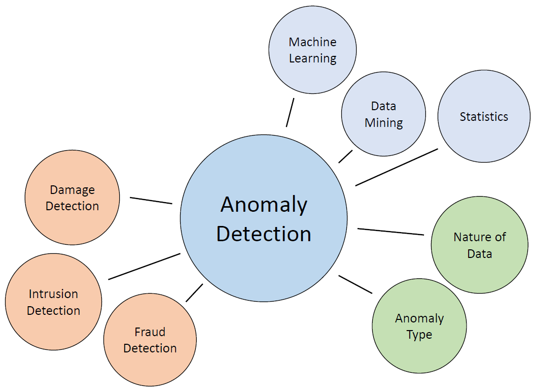
Anomaly detection is a crucial technique in data analysis, with applications ranging from fraud detection to network security. It involves identifying unusual data points that deviate significantly from the majority of observations. In this tutorial, we will explore the concept of anomaly detection and demonstrate how to implement it using Python. Specifically, we’ll use the Isolation Forest algorithm, a powerful method for anomaly detection.
Understanding Anomaly Detection: Anomalies, or outliers, are data points that behave differently from the norm. They can be categorized into three types:
Point Anomaly: A single data point that stands out significantly from the rest of the data.
Contextual Anomaly: An observation is considered anomalous based on its context.
Collective Anomaly: A group of data instances collectively contributes to identifying an anomaly.
Anomaly detection can be accomplished using machine learning techniques, and we’ll explore two common approaches: supervised and unsupervised.
Supervised Anomaly Detection: In supervised anomaly detection, we use a labeled dataset containing both normal and anomalous samples to train a predictive model. Common algorithms for this approach include Neural Networks, Support Vector Machine (SVM), and K-Nearest Neighbors (KNN) Classifier.
Unsupervised Anomaly Detection: Unsupervised anomaly detection, on the other hand, does not require labeled training data. It operates under the assumptions that only a small percentage of data is anomalous, and anomalies are statistically different from normal data points. Unsupervised methods cluster data based on similarity and identify data points far from these clusters as anomalies.
Implementing Anomaly Detection with Isolation Forest:
Now, let’s dive into a Python code example to perform anomaly detection using the Isolation Forest algorithm, which is available in the pyod (Python Outlier Detection) library.
Step 1: Importing Libraries
import numpy as np
from scipy import stats
import matplotlib.pyplot as plt
from pyod.models.knn import KNN
from pyod.utils.data import generate_data, get_outliers_inliers
Step 2: Creating Synthetic Data
# Generate a random dataset with two features
X_train, y_train = generate_data(n_train=300, train_only=True, n_features=2)
# Set the percentage of outliers
outlier_fraction = 0.1
# Separate outliers and inliers
X_outliers, X_inliers = get_outliers_inliers(X_train, y_train)
n_inliers = len(X_inliers)
n_outliers = len(X_outliers)
# Separate the two features
f1 = X_train[:, [0]].reshape(-1, 1)
f2 = X_train[:, [1]].reshape(-1, 1)
Step 3: Visualizing the Data
# Create a meshgrid
xx, yy = np.meshgrid(np.linspace(-10, 10, 200), np.linspace(-10, 10, 200))
# Scatter plot
plt.scatter(f1, f2)
plt.xlabel(‘Feature 1’)
plt.ylabel(‘Feature 2’)
Step 4: Training and Evaluating the Model
# Train the Isolation Forest model
clf = KNN(contamination=outlier_fraction)
clf.fit(X_train, y_train)
# Calculate prediction scores
scores_pred = clf.decision_function(X_train) * -1
# Predict anomalies
y_pred = clf.predict(X_train)
n_errors = (y_pred != y_train).sum()
print(‘The number of prediction errors is ‘ + str(n_errors))
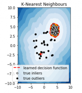
Step 5: Visualizing the Predictions
# Set a threshold to consider a datapoint as an inlier or outlier
threshold = stats.scoreatpercentile(scores_pred, 100 * outlier_fraction)
# Calculate decision function scores for the meshgrid
Z = clf.decision_function(np.c_[xx.ravel(), yy.ravel()]) * -1
Z = Z.reshape(xx.shape)
# Create a contour plot
subplot = plt.subplot(1, 2, 1)
subplot.contourf(xx, yy, Z, levels=np.linspace(Z.min(), threshold, 10), cmap=plt.cm.Blues_r)
# Draw a red contour line where anomaly score is equal to the threshold
a = subplot.contour(xx, yy, Z, levels=[threshold], linewidths=2, colors=’red’)
# Create orange contour lines where anomaly score ranges from threshold to maximum anomaly score
subplot.contourf(xx, yy, Z, levels=[threshold, Z.max()], colors=’orange’)
# Scatter plot of inliers with white dots
b = subplot.scatter(X_train[:-n_outliers, 0], X_train[:-n_outliers, 1], c=’white’, s=20, edgecolor=’k’)
# Scatter plot of outliers with black dots
c = subplot.scatter(X_train[-n_outliers:, 0], X_train[-n_outliers:, 1], c=’black’, s=20, edgecolor=’k’)
subplot.axis(‘tight’)
subplot.legend([a.collections[0], b, c], [‘Learned Decision Function’, ‘True Inliers’, ‘True Outliers’],
loc=’lower right’, prop=plt.matplotlib.font_manager.FontProperties(size=10))
subplot.set_title(‘K-Nearest Neighbors’)
subplot.set_xlim((-10, 10))
subplot.set_ylim((-10, 10))
plt.show()
Conclusion:
In this tutorial, we’ve explored the concept of anomaly detection and implemented it using the Isolation Forest algorithm in Python. Anomaly detection is a critical technique with applications in various domains, and Isolation Forest is just one of the many algorithms available for this purpose. Depending on your specific use case and data, you can explore different methods to effectively identify anomalies and address potential issues or threats in your data.
Next Steps:
Apply anomaly detection techniques to your own datasets or real-world problems.
Experiment with different algorithms and parameters for optimal anomaly detection.
Integrate anomaly detection into your data pipelines for real-time monitoring and decision-making.
Stay vigilant, as anomaly detection is a valuable tool for maintaining data integrity and security in a wide range of applications.